Quickstart
In this tutorial we show how to obtain a mock-catalogue using
scampy.
First, we will load a DM halo/sub-halo hierarchy obtained with the SUBFIND algorithm applied on a \(z = 0\) GADGET snapshot. Then, we will
populate the catalogue with galaxies
associate to each galaxy a luminosity
First of all, we populate the namespaces from numpy and matplotlib (it
would be enough to state import numpy as np for working, this is
mostly useful for plotting)
import numpy as np
# %pylab inline
Now, we import the catalogue module from scampy:
from scampy import catalogue
We now build an object of type catalogue and read the halo/sub-halo hierarchy from the binary output of the SUBFIND algorithm.
Note that, tipically, these outputs are given as a set of files with
a common base-name, e.g. subhalo_tab.0 for the first file in the
set. Here we just need to provide the common name of all the files, i.e.
subhalo_tab.
cat = catalogue.catalogue()
cat.read_hierarchy_from_gadget( "input/subhalo_tab" )
The catalogue we provide in the input directory has been obtained
for a simulation box with side-lenght
\(L_\text{box} = 512\ \text{Mpc}/h\), thus we can define a
volume variable that we will use later:
volume = 512**3
1. Populate catalogue
We will now populate the above catalogue with a 4-parameters HOD model:
with parameters: \(A_\text{min} = 10^{14}\ M_\odot/h\), \(\sigma_{\log A} = 0.5\), \(A_\text{sat} = 10^{15}\ M_\odot/h\) and \(\alpha_\text{sat} = 1\).
To do so, we have first to build an object of type occupation_p with
given parameters:
from scampy import occupation_p
ocp = occupation_p.tinker10_p( Amin = 1.e+14, siglogA = 0.5, Asat=1.e+15, alpsat=1. )
Then, we can call the populate function of the class catalogue,
which returns a populated catalogue:
gxy_cat = cat.populate( ocp )
In order to get the number of hosted galaxies we can use the dedicated function of the class catalogue:
Ng = gxy_cat.Nhost()
2. Associate luminosity
In order to run the SHAM algorithm, we import the abundance_matching
module of scampy
from scampy import abundance_matching
First of all, we need the probability distribution of the observable we want to add to the mock galaxies.
Le us define a Schechter luminosity function:
def schechter ( mag ) :
    alpha = -1.07
    norm = 1.6e-2
    mstar = -19.7 + 5. * np.log10( 5. )
    lum = - 0.4 * ( mag - mstar )
    # this to control overflow when integrating:
    if lum > 308. : lum = 308.
    return 0.4 * np.log( 10 ) * norm * 10**( - 0.07 * lum ) * np.exp( - 10**lum )
The routine that implements the SHAM algorithm operates on arrays of
galaxy type objects, instead of on objects of type catalogue.
Such arrays can be extracted from a populated catalogue either directly,
by calling the populate() function with the argument
extract = True:
galaxies = cat.populate( ocp, extract = True )
or by calling the extract_galaxies() function of the catalogue
module. This function takes 2 arguments:
an array of
host_halotype objects (i.e. thecontentof a catalogue;the number of galaxies found by the
populatealgorithm.
galaxies = catalogue.extract_galaxies( gxy_cat.content, Ng )
At this point we have everything we need for running the SHAM algorithm.
It is implemented in the abundance_matching() function of the
abundance_matching module. This function takes several argumens, we
refer the reader to the documentation for a detailed description.
The positional arguments are:
the array of
galaxytype objects (galaxies);the probability distribution of the observable property we want to match (it must depend only on one-variable).
Here we are also setting the following keyword arguments:
minLandmaxL, the limits of the free-variable in our probability distribution;nbinM, the number of bins we want to divide the mass-space;factM, the constant factor to multiply the mass-distribution (since we want a volume density, here we are passing1/volume.
galaxies = abundance_matching.abundance_matching( galaxies, schechter,
                                                  minL = -20, maxL = -10,
                                                  nbinM = 20, factM = 1. / volume )
… and that’s all folks!
The galaxies array now contains all the mock-galaxies of our
catalogue.
Analysis
Here we show some results from measures that can be performed on the populated catalogue.
First of all, let us populate the matplotlib and numpy namespaces …
%pylab inline
Populating the interactive namespace from numpy and matplotlib
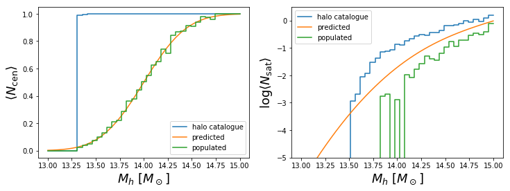
Abundances
We will plot here histograms of the average number of central and satellite haloes per mass-bin, compared with the occupation predicted by the selected model and with the average number of central and satellite mock galaxies in the output catalogue.
Define the log-spaced mass bins:
ms_binned = np.logspace( +13, +15, 40 )
Get abundances of the halo catalogue:
Nc_hal, Ns_hal = catalogue.get_abundances( cat, ms_binned )
Get abundances of the galaxy catalogue:
Nc_gxy, Ns_gxy = catalogue.get_abundances( gxy_cat, ms_binned )
Plot:
fig = plt.figure( figsize = ( 12, 4 ) )
ax1 = fig.add_subplot( 121 )

ax1.set_xlabel('$M_h$ $[M_\\odot]$', fontsize=18)
ax1.set_ylabel('$\\langle N_\\mathrm{cen} \\rangle$', fontsize=18)

ax1.step( np.log10( ms_binned ), Nc_hal,
          label = 'halo catalogue' )
ax1.plot( np.log10( ms_binned ), [ ocp.Ncen( mm ) for mm in ms_binned ],
          label = 'predicted' )
ax1.step( np.log10( ms_binned ), Nc_gxy,
          label = 'populated' )

ax1.legend()

ax2 = fig.add_subplot( 122 )

ax2.set_ylim( [ -5, 0.5 ] )
ax2.set_xlabel('$M_h$ $[M_\\odot]$', fontsize=18)
ax2.set_ylabel('$\\log \\langle N_\\mathrm{sat} \\rangle$', fontsize=18)

ax2.step( np.log10( ms_binned ), np.log10( Ns_hal + 1.e-7 ),
          label = 'halo catalogue' )
ax2.plot( np.log10( ms_binned ), np.log10( [ ocp.Nsat( mm ) for mm in ms_binned ] ),
          label = 'predicted' )
ax2.step( np.log10( ms_binned ), np.log10( Ns_gxy + 1.e-7 ),
          label = 'populated' )

ax2.legend()
<matplotlib.legend.Legend at 0x7f897235c518>
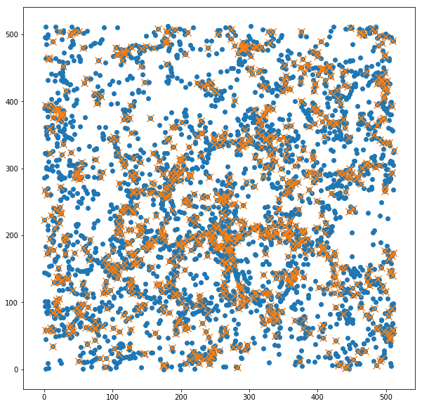
Simulation box:
To have an idea of how the original halo catalogue has been trimmed by the HOD prescription, we show here a slice of the simulation box with positions of the haloes and mock galaxies.
Extract the halo coordinates from the original catalogue and select a \(64\ \text{Mpc}/h\) slice along the z-axis:
coords_hal = np.concatenate( ( cat.get_coord_cen(), cat.get_coord_sat() ) ).T
wz_hal = np.where( [ ( 224. < _z ) & ( _z < 288. ) for _z in coords_hal[ 2 ] ] )
Extract the halo coordinates from the populated catalogue and select a \(64\ \text{Mpc}/h\) slice along the z-axis:
coords_gxy = np.concatenate( ( gxy_cat.get_coord_cen(), gxy_cat.get_coord_sat() ) ).T
wz_gxy = np.where( [ ( 224. < _z ) & ( _z < 288. ) for _z in coords_gxy[ 2 ] ] )
Plot the slice:
figure( figsize = ( 10, 10 ) )

pyplot.scatter( coords_hal[ 0 ][ wz_hal ], coords_hal[ 1 ][ wz_hal ] )
pyplot.scatter( coords_gxy[ 0 ][ wz_gxy ], coords_gxy[ 1 ][ wz_gxy ], marker='x', s = 100 )
<matplotlib.collections.PathCollection at 0x7f8970d4a8d0>
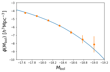
Luminosity function:
Finally, we want to see what is the luminosity distribution of the
output galaxy mock catalogue. Let us store the luminosities of all the
mock galaxies into a numpy array:
luminosities = np.array( [ gxy.luminosity for gxy in galaxies ] )
We will now call the cumulative_counts function of the
abundance_matching module. This function is also used internally by
the function that applies the SHAM prescription. Internally, it counts
the number of occurrencies in an array with value greater than some
fixed quantity, therefore, we have to invert the magnitudes sign to make
it work:
mag_mes = np.linspace( -19., -17., 10 )
phi_mes, phi_mes_er = abundance_matching.cumulative_counts( -1 * luminosities, -1 * mag_mes, 1. / volume )
We can now plot the result, along with the integrated Schechter
luminosity function. The latter can be obtained with the utility
function cumulative_from_differential of the abundance_matching
module:
plt.xlabel( '$M_\mathrm{bol}$', fontsize = 18 )
plt.ylabel( '$\phi( M_\mathrm{bol} )\ [h^3 \mathrm{Mpc}^{-3}]$', fontsize = 18 )

plt.xlim( [ -17.5, -19.2 ] )
plt.ylim( [ -10, -3 ] )

size = 30
MM = np.linspace( -21, -16., size )

plot( MM, np.log10( abundance_matching.cumulative_from_differential( schechter, MM ) ) )
errorbar( mag_mes, np.log10( phi_mes ),
          yerr = phi_mes_er / phi_mes, fmt = 'o' )
<ErrorbarContainer object of 3 artists>