Welcome to ScamPy’s documentation!

A Python interface for Sub-halo Clustering and Abundance Matching

ScamPy is a highly-optimized and flexible library for “painting” an observed population of cosmological objects on top of the DM-halo/subhalo hierarchy obtained from DM-only simulations. The method used combines the classical Halo Occupation Distribution (HOD) with the sub-halo abundance matching (SHAM), the sinergy of the two processes is dubbed Sub-halo clustering and abundance matching (SCAM). The procedure itself is quite easy since it only requires to apply the two methods in sequence:

1. by applying the HOD scheme, the host sub-haloes are selected;

2. the SHAM algorithm associates to each sub-halo an observable property of choice.

What can be achieved

Here is an animation obtained by running ScamPy on the halo/subhalo catalogues of 42 different snapshots, from redshift z=8 to redshift z=0, of the same \(64 Mpc/h\) DM-only N-body simulation. The simulation has been obtained with the non-public code GADGET-3, following the evolution of \(512^3\) DM particles. For each different redshift we have fixed the parameters values for the HOD and matched the UV-luminosity function of star-forming galaxies.

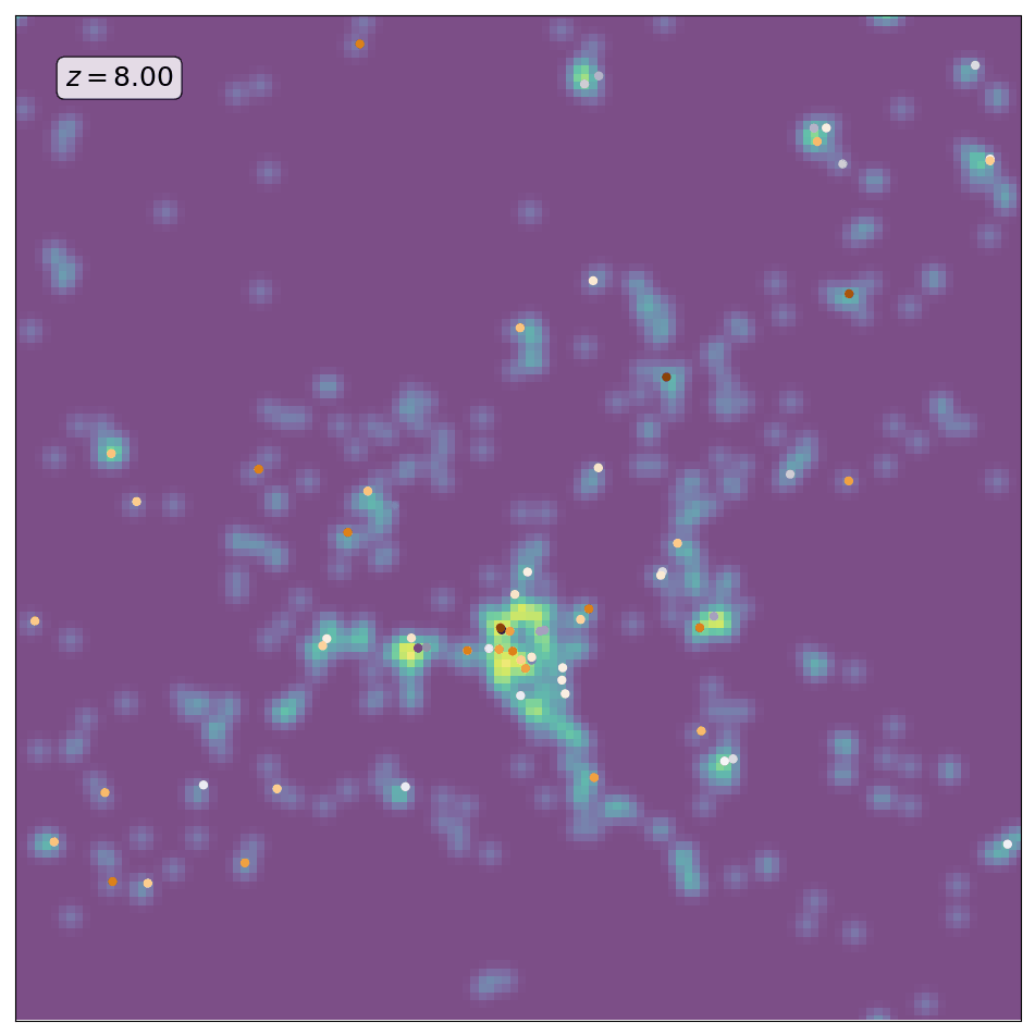
The background color-code shows the underlying DM-density field computed by smoothing the contribution of DM-particles in a 10 Mpc/h thick slice of the simulation. The markers locate the positions of the mock galaxies generated with ScamPy. Circles mark the position of the central galaxies while crosses mark the position of satellite galaxies. The marker color represents lower to higher luminosity going from brighter to darker.

Basic Usage

If you wanted to populate a DM catalogue with galaxies with given luminosity, you would do something like:

# read the sub-halo catalogue from a file
from scampy import catalogue
cat = catalogue.catalogue()
cat.read_hierarchy_from_gadget( "/path/to/input_directory/subhalo_tab_snap" )
volume = 512.**3 # for a box with side-lenght = 512 Mpc/h


# build an object of type occupation probability with given parameters
from scampy import occupation_p
ocp = occupation_p.tinker10_p( Amin    = 1.e+14,
                               siglogA = 0.5,
                               Asat    = 1.e+15,
                               alpsat  = 1. )

# populate the catalogue
galaxies = cat.populate( ocp, extract = True )

# define a Schechter-like luminosity function
import numpy as np
def schechter ( mag ) :
     alpha = -1.07
     norm = 1.6e-2
     mstar = -19.7 + 5. * np.log10( 5. )
     lum = - 0.4 * ( mag - mstar )
     return 0.4 * np.log( 10 ) * norm * 10**( - 0.07 * lum ) * np.exp( - 10**lum )

# call the sub-halo abundance matching routine:
from scampy import abundance_matching
galaxies = abundance_matching.abundance_matching( galaxies, schechter, factM = 1. / volume )

The galaxies array contains the output mock-galaxies.

Installation guide

Installation of ScamPy is dealt by the Meson Build System. Each module of the API is built by a specific meson.build script.

You can decide to install it either in - developer-mode, with shared libraries for the C/C++ sectors and headers organized in the

POSIX directory structure (libraries in lib, headers in include, python package in lib/pythonX.Y/site-packages)

• package-mode, with the C++ sector compiled into static libraries within an internal sub-module of the package and C-wrapping compiled dynamically along with the former. This is what you would obtain by pip-installing from the root directory of the project.

developer-mode Install

From the root directory of this repository run

meson build_dir --prefix /path/to/install_directory
meson install -C build_dir

If no --prefix is specified the library will be installed in the system default prefix directory (usually /usr/local).

package-mode Install

From the root directory of this repository either run

meson build_dir --prefix /path/to/install_directory -Dfull-build=false
meson install -C build_dir

or run

In the latter case the standard path for the python installation directory will be used.

Meson options

• full-build: boolean, enables/disables the full build installation.

• enable-doc: boolean, enables/disables building of the documentation. If enabled, docs will appear in the $PREFIX/share/man directory

• enable-test: boolean, enables/disables testing (to run tests after having compiled the project run meson test -C build_dir from the root directory of this repository)

Pre-requisites

For building:

• meson<0.57 build system tool

• ninja

can both be installed either via conda install or with pip install

Warning

The current latest version of meson (i.e. 0.57.2) does not always support compiling heritage fortran programs (typically an error of type UnicodeDecodeError is raised). If the external library FFTLog (see below) is not already installed in your system (and visible to the linker), the installation process will try to download and compile it with ninja. If your meson version is superior to 0.56.2 this will cause a failure in the installation process. The quickest fix is to downgrade your build system tool to meson<=0.56.2.

Dependencies of the library:

• GNU Scientific Library version 2 or greater (GSL link);

• FFTLog (FFTLog link).

While GSL has to be already installed in the system, if FFTLog is not present Meson will authomatically download it along with a patch we have developed, both will be installed in the subprojects directory of the repository.

Dependencies for building the documentation locally:

• Doxygen

• Sphynx (with breathe, autodoc and rtd_theme extensions)

Note

A YAML file containing the specs for building a conda environment with all the dependencies needed to build the docs is available at doc_environment.yml

Dependencies for enabling testing:

• Google Test (is authomatically installed by Meson)

Python Documentation

interpolator module

cosmology module

occupation_p module

halo_model module

gadget_file module

class scampy.gadget_file.gadget_file(filebase, byteorder='little', ids_lenght=8, masstab=True)

A class for reading GaDGET SUBFIND subgroup tables

Parameters

• filebase (string) – common name of the files to be read

• byteorder (string) – ‘little’ or ‘big’ for little or big endian, respectively

• ids_lenght (int) – number of bytes of the integer storing the IDs (8 or 16)

• masstab (bool) – whether the file contains mass tables

read_file(num, scale_mass=10000000000.0, scale_lenght=0.001, add_to_internal=False, verbose=False)

Reads the num`^th file in `base

Parameters

• num (int) – file to read

• scale_mass (float) – mass unit (in terms of solar masses, default = 1.e+10)

• scale_lenght (float) – lenght unit (in terms of Mpc/h, default = 1.e-3)

• add_to_internal (bool) – whether to add the data to the internal storage array of the class (default = False)

• verbose (bool) – whether to print on screen additional info (default = False)

Returns

Return type

None

read_header(num=0)

Reads only the Header of the num`^th file in `base

Parameters

num (the file number to read) –

Returns

• loc (dictionary with meta-data local to file num)

• glob (dictionary with meta-data global to all files in base)

objects module

catalogue module

scampy.catalogue.extract_galaxies(hhaloes, ngxy)

Extracts objects of type galaxy from an host halo catalogue :param hhaloes: :type hhaloes: the input host-halo catalogue :param ngxy: in the input catalogue :type ngxy: the number of galaxies hosted by all the host haloes

Returns

Return type

numpy array containing ngxy galaxies

class scampy.catalogue.catalogue(X=None, scale_lenght=0.001, scale_mass=10000000000.0, boxsize=None)

Class to handle catalogues of objects of type halo, host_halo, galaxy

Nhost(mask=None)

Return the total number of host haloes (central + satellites)

Parameters

mask (array-like) – Array mask for filtering the original catalogue

Returns

Return type

int

get_coord_cen(store=False)

Get the coordinates of all the central objects in the catalogue

Parameters

store (whether to store the returned array into an internal variable ( default = False )) –

Returns

Return type

Array of central objects coordinates ( shape = ( n_central, 3 ) )

get_coord_sat(store=False)

Get the coordinates of all the satellite objects in the catalogue

Parameters

store (whether to store the returned array into an internal variable ( default = False )) –

Returns

Return type

Array of satellite objects coordinates ( shape = ( n_satellites, 3 ) )

get_mass_cen(store=False)

Get the masses of all the central objects in the catalogue

Parameters

store (whether to store the returned array into an internal variable ( default = False )) –

Returns

Return type

Array of central objects mass ( shape = ( n_central, 3 ) )

get_mass_halo(store=False)

Get the masses of

Parameters

store (bool) – whether to store the returned array into an internal variable ( default = False )

Returns

Return type

Array of ( shape = ( , 3 ) )

get_mass_sat(store=False)

Get the masses of all the satellite objects in the catalogue

Parameters

store (whether to store the returned array into an internal variable ( default = False )) –

Returns

Return type

Array of satellite objects mass ( shape = ( n_satellites, 3 ) )

read_hierarchy_from_gadget(filebase, boxsize=None)

Reads the halo/sub-halo hierarchy from a Subgroup gadget output

Parameters

filebase –

Returns

Return type

None

set_content(X)

Add element(s) to the catalogue

Parameters

X (array-like) –

Returns

Return type

None

sub_sample(nsample)

Return a sub-sampled catalogue

Parameters

nsample (int) – number of objects in the sub-sampled catalogue, must be in the interval [0.,Nhost) where Nhost is the number of sub-haloes of the current catalogue

Returns

sub-sampled copy of the original catalogue

Return type

catalogue

abundance_matching module

Quickstart

In this tutorial we show how to obtain a mock-catalogue using scampy.

First, we will load a DM halo/sub-halo hierarchy obtained with the SUBFIND algorithm applied on a \(z = 0\) GADGET snapshot. Then, we will

1. populate the catalogue with galaxies

2. associate to each galaxy a luminosity

First of all, we populate the namespaces from numpy and matplotlib (it would be enough to state import numpy as np for working, this is mostly useful for plotting)

import numpy as np
# %pylab inline

Now, we import the catalogue module from scampy:

from scampy import catalogue

We now build an object of type catalogue and read the halo/sub-halo hierarchy from the binary output of the SUBFIND algorithm.

Note that, tipically, these outputs are given as a set of files with a common base-name, e.g. subhalo_tab.0 for the first file in the set. Here we just need to provide the common name of all the files, i.e. subhalo_tab.

cat = catalogue.catalogue()
cat.read_hierarchy_from_gadget( "input/subhalo_tab" )

The catalogue we provide in the input directory has been obtained for a simulation box with side-lenght \(L_\text{box} = 512\ \text{Mpc}/h\), thus we can define a volume variable that we will use later:

volume = 512**3

1. Populate catalogue

We will now populate the above catalogue with a 4-parameters HOD model:

with parameters: \(A_\text{min} = 10^{14}\ M_\odot/h\), \(\sigma_{\log A} = 0.5\), \(A_\text{sat} = 10^{15}\ M_\odot/h\) and \(\alpha_\text{sat} = 1\).

To do so, we have first to build an object of type occupation_p with given parameters:

from scampy import occupation_p
ocp = occupation_p.tinker10_p( Amin = 1.e+14, siglogA = 0.5, Asat=1.e+15, alpsat=1. )

Then, we can call the populate function of the class catalogue, which returns a populated catalogue:

gxy_cat = cat.populate( ocp )

In order to get the number of hosted galaxies we can use the dedicated function of the class catalogue:

Ng = gxy_cat.Nhost()

2. Associate luminosity

In order to run the SHAM algorithm, we import the abundance_matching module of scampy

from scampy import abundance_matching

First of all, we need the probability distribution of the observable we want to add to the mock galaxies.

Le us define a Schechter luminosity function:

def schechter ( mag ) :
    alpha = -1.07
    norm = 1.6e-2
    mstar = -19.7 + 5. * np.log10( 5. )
    lum = - 0.4 * ( mag - mstar )
    # this to control overflow when integrating:
    if lum > 308. : lum = 308.
    return 0.4 * np.log( 10 ) * norm * 10**( - 0.07 * lum ) * np.exp( - 10**lum )

The routine that implements the SHAM algorithm operates on arrays of galaxy type objects, instead of on objects of type catalogue.

Such arrays can be extracted from a populated catalogue either directly, by calling the populate() function with the argument extract = True:

galaxies = cat.populate( ocp, extract = True )

or by calling the extract_galaxies() function of the catalogue module. This function takes 2 arguments:

• an array of host_halo type objects (i.e. the content of a catalogue;

• the number of galaxies found by the populate algorithm.

galaxies = catalogue.extract_galaxies( gxy_cat.content, Ng )

At this point we have everything we need for running the SHAM algorithm. It is implemented in the abundance_matching() function of the abundance_matching module. This function takes several argumens, we refer the reader to the documentation for a detailed description.

The positional arguments are:

• the array of galaxy type objects (galaxies);

• the probability distribution of the observable property we want to match (it must depend only on one-variable).

Here we are also setting the following keyword arguments:

• minL and maxL, the limits of the free-variable in our probability distribution;

• nbinM, the number of bins we want to divide the mass-space;

• factM, the constant factor to multiply the mass-distribution (since we want a volume density, here we are passing 1/volume.

galaxies = abundance_matching.abundance_matching( galaxies, schechter,
                                                  minL = -20, maxL = -10,
                                                  nbinM = 20, factM = 1. / volume )

… and that’s all folks!

The galaxies array now contains all the mock-galaxies of our catalogue.

Analysis

Here we show some results from measures that can be performed on the populated catalogue.

First of all, let us populate the matplotlib and numpy namespaces …

%pylab inline

Populating the interactive namespace from numpy and matplotlib

Abundances

We will plot here histograms of the average number of central and satellite haloes per mass-bin, compared with the occupation predicted by the selected model and with the average number of central and satellite mock galaxies in the output catalogue.

Define the log-spaced mass bins:

ms_binned = np.logspace( +13, +15, 40 )

Get abundances of the halo catalogue:

Nc_hal, Ns_hal = catalogue.get_abundances( cat, ms_binned )

Get abundances of the galaxy catalogue:

Nc_gxy, Ns_gxy = catalogue.get_abundances( gxy_cat, ms_binned )

Plot:

fig = plt.figure( figsize = ( 12, 4 ) )
ax1 = fig.add_subplot( 121 )

ax1.set_xlabel('$M_h$ $[M_\\odot]$', fontsize=18)
ax1.set_ylabel('$\\langle N_\\mathrm{cen} \\rangle$', fontsize=18)

ax1.step( np.log10( ms_binned ), Nc_hal,
          label = 'halo catalogue' )
ax1.plot( np.log10( ms_binned ), [ ocp.Ncen( mm ) for mm in ms_binned ],
          label = 'predicted' )
ax1.step( np.log10( ms_binned ), Nc_gxy,
          label = 'populated' )

ax1.legend()

ax2 = fig.add_subplot( 122 )

ax2.set_ylim( [ -5, 0.5 ] )
ax2.set_xlabel('$M_h$ $[M_\\odot]$', fontsize=18)
ax2.set_ylabel('$\\log \\langle N_\\mathrm{sat} \\rangle$', fontsize=18)

ax2.step( np.log10( ms_binned ), np.log10( Ns_hal + 1.e-7 ),
          label = 'halo catalogue' )
ax2.plot( np.log10( ms_binned ), np.log10( [ ocp.Nsat( mm ) for mm in ms_binned ] ),
          label = 'predicted' )
ax2.step( np.log10( ms_binned ), np.log10( Ns_gxy + 1.e-7 ),
          label = 'populated' )

ax2.legend()

<matplotlib.legend.Legend at 0x7f897235c518>

Simulation box:

To have an idea of how the original halo catalogue has been trimmed by the HOD prescription, we show here a slice of the simulation box with positions of the haloes and mock galaxies.

Extract the halo coordinates from the original catalogue and select a \(64\ \text{Mpc}/h\) slice along the z-axis:

coords_hal = np.concatenate( ( cat.get_coord_cen(), cat.get_coord_sat() ) ).T
wz_hal = np.where( [ ( 224. < _z ) & ( _z < 288. ) for _z in coords_hal[ 2 ] ] )

Extract the halo coordinates from the populated catalogue and select a \(64\ \text{Mpc}/h\) slice along the z-axis:

coords_gxy = np.concatenate( ( gxy_cat.get_coord_cen(), gxy_cat.get_coord_sat() ) ).T
wz_gxy = np.where( [ ( 224. < _z ) & ( _z < 288. ) for _z in coords_gxy[ 2 ] ] )

Plot the slice:

figure( figsize = ( 10, 10 ) )

pyplot.scatter( coords_hal[ 0 ][ wz_hal ], coords_hal[ 1 ][ wz_hal ] )
pyplot.scatter( coords_gxy[ 0 ][ wz_gxy ], coords_gxy[ 1 ][ wz_gxy ], marker='x', s = 100 )

<matplotlib.collections.PathCollection at 0x7f8970d4a8d0>

Luminosity function:

Finally, we want to see what is the luminosity distribution of the output galaxy mock catalogue. Let us store the luminosities of all the mock galaxies into a numpy array:

luminosities = np.array( [ gxy.luminosity for gxy in galaxies ] )

We will now call the cumulative_counts function of the abundance_matching module. This function is also used internally by the function that applies the SHAM prescription. Internally, it counts the number of occurrencies in an array with value greater than some fixed quantity, therefore, we have to invert the magnitudes sign to make it work:

mag_mes = np.linspace( -19., -17., 10 )
phi_mes, phi_mes_er = abundance_matching.cumulative_counts( -1 * luminosities, -1 * mag_mes, 1. / volume )

We can now plot the result, along with the integrated Schechter luminosity function. The latter can be obtained with the utility function cumulative_from_differential of the abundance_matching module:

plt.xlabel( '$M_\mathrm{bol}$', fontsize = 18 )
plt.ylabel( '$\phi( M_\mathrm{bol} )\ [h^3 \mathrm{Mpc}^{-3}]$', fontsize = 18 )

plt.xlim( [ -17.5, -19.2 ] )
plt.ylim( [ -10, -3 ] )

size = 30
MM = np.linspace( -21, -16., size )

plot( MM, np.log10( abundance_matching.cumulative_from_differential( schechter, MM ) ) )
errorbar( mag_mes, np.log10( phi_mes ),
          yerr = phi_mes_er / phi_mes, fmt = 'o' )

<ErrorbarContainer object of 3 artists>

Indices and tables

• Index

• Module Index

• Search Page